Material: Concrete
Soiling: Algae, lichens, mosses
Cleaning technique: Cold-water high-pressure cleaning
Transient art conjured on harbor wall
Together with Kärcher, artist Klaus Dauven created a transient work of art on the fishing port’s harbor wall of Southern French town of Sète.
On the fishing port’s harbor wall of Southern French town of Sète, artist Klaus Dauven created a transient work of art together with Kärcher. The artwork depicts the faces of local characters, created in the so called reverse graffiti method.
“Reverse graffiti” forms subjects by the precise removal of organic soiling like algae, lichens and mosses.
Local characters perpetuated
The port town’s and pier’s long history inspired the artist’s subjects: he chose different local personalities with ties to the shipping or fishing industry, who have especially expressive faces.
Saint Louis, the 650 meter long pier built in 1666, was the first structure in the town of Sète.


Multiplex panels, which Klaus Dauven prepared in advance, served as stencils.

With the help of a petrol-powered cold water high pressure cleaner of the type HD 9/23 G, the harbor wall was cleaned all around the stencils.

The subjects emerge as a result of the light-dark contrast between the cleaned and the untreated surfaces.

Large yachts visiting Sète
One of the town’s largest maritime festivals took place simultaneously to the cleaning work at the pier. More than 100 boats and yachts are docked in the harbor for the “Escale”, including France’s most beautiful windjammers – a fitting backdrop for the new works of art along the pier
The French town Sète lies at the Eastern end of the approximately 16 kilometer long headland “Le Toc”. The most important French fishing harbor in the Mediterranean lies here right next to the town center
Methods for depicting a harbor
Results and Discussion
Quartermaster Harbor is a popular area fpr research done by University of Washington professors and students, due to presence of Alexandrium cantenella which causes paralytic shellfish poisoning (PSP). Data collected by the Estuary Field Couse in the Spring quarter of 2009 will be compared to past research in the summary section, as well as used by future researchers for comparison.
This results and discussion section is limited to graphs, for more in depth data click on the data repository page, located on the left tool bar.

Quartermaster Harbor Map (Click to enlarge)
Comparison of Methods
Click to enlarge
Above are correlation curves that explain the variation difference between the two methods used to interpret dissolved oxygen and fluorescence data. The first method was collected using a CTD and the second method was physically collected using Nisken and Thoreson Bottles. By plotting the two different methods againist each other,the quality of data is observed by analyzing the best fit line.
An equation is constructed by the best fit line and present on the graphs above. The R^2 value represents the variation between the two different methods used to collect the data.
Click to enlarge
Figure 1: CTD surfer plot depicting the temperature (deg C) variations shown by horizontal lines at different depths. The plot shows on the (Y) axis the depth (m) and on the (X) axis distance (km).
The CTD plot above displays temperature range according to depth depicted by shades of blue. Stations with deeper depths have cooler temperatures shown with darker shades of blue, while stations with shallower depths have warmer surface temperatures with lighter shades of blue. The correlation shown in the plot, displays deeper depths having a characteristic of cooler surface temperatures. Surface temperatures do not begin to increase rapidly until station 52.
Click to enlarge
Figure 2: CTD surfer plot depicting the fluorescence (ug/L) concentrations by horizontal lines at different depths. The plot shows on the (Y) axis the depth (m) and on the (X) axis distance (km).
The CTD plot above shows fluorescence (ug/L) at higher concentrations corresponding with darker shades of green, while lighter shades of green depict lower concentrations. Surfer plot shows that Quartermaster Harbor has higher concentrations of fluorescence dominant at depth range of 4-10m.
Fluorescence analysis of data, shown in Figure 2, contains interesting findings of no visible solid trend. Higher concentrations of fluorescence is a direct correlation to phytoplankton productivity. Station 50 and 51 have expectable results. Station 50 exhibits an increase in chlorophyll at the thermocline of 4m and then proceeds into a decrease further in depth below the surface. Station 51 has similar characteristics of station 50, however the higher concentration of fluorescence spans a deeper depth. Proceeding to station 52, the surfer plot shows a patch of higher concentration at depths of 8-12m. This higher concentration of fluorescence is deeper than the thermocline. Station 53 shows similar characteristics as station 50, where higher concentration of fluorescence is present at the thermocline. Stations 54 and 55, show a patch of higher concentration of fluorescence at depths of 5-8m. This characteristic is similar to station 52, in which the high concentration is deeper than thermocline. Station 56 is the shallower of all the stations and shows a characteristic of increasing fluorescence as depth increases. All stations that show a higher concentration of fluorescence at the thermocline is due to the fact that this is prime real estate for phytoplankton. Higher concentrations of fluorescence lower than thermocline depth is not easily explained.
Transmissivity
Click to enlarge
Figure 3: CTD surfer plot depicting transmissivity levels (%) by horizontal lines at different depths. The plot shows on the (Y) axis the depth (m) and on the (X) axis distance (km).
The CTD plot above shows the transmissivity levels (%) at higher visibility corresponding with lighter shades of yellow, while lower visibility corresponds with darker shades of yellow. The surfer plot above shows opaqueness at station 50 increasing with depth. Highest percent of visibility is shown at surface depths at station 52 and 53. Station 52 contains a patch of higher visibilty at 11m, which is unexplainable. The opaque hook at station 53 is, as well, unexplainable. All other stations show an decrease in visibility as depth increases. This pattern is expected due to the solar absorption.
Dissolved Oxygen
Click to enlarge
Figure 4: CTD surfer plot depicting the dissolved oxygen levels (mg/L) by horizontal lines at different depths. The plot shows on the (Y) axis the depth (m) and on the (X) axis distance (km).
The CTD plot above shows the higher concentrations of dissolved oxygen with darker shade of orange. Lower concentrations are correlated to lighter shades of orange. Overlooking the oddity of oxygen depletion at station 52’s bottom depth, a common trend of higher dissolved oxygen at the surface is visible at all stations. Due to the expected trend, concentration of dissolved oxygen decrease as depth increases at all stations. Another variable effecting dissolved oxygen is the temperature and high bioproductivity. The higher temperature and high bioproductivity decrease the hold of gas from the water, resulting in a lesser ability to hold oxygen.
Click to enlarge
Figure 5: CTD surfer plot depicting the salinity (PSU) by horizontal lines at different depths. The plot shows on the (Y) axis the depth (m) and on the (X) axis distance (km).
The CTD plot above shows the higher concentrations of salinity with darker shade of red. Lower concentrations are correlated to lighter shades of red. The salinity data above shows a trend that would be expected from fresh water influx/ Stations 50 and 51 are further out in the sound and have lower concentration of salinity at lower surface depths. Stations 52 through 56 are influenced by fresh water influx and result in a higher concentration of salinity at surface depths. All stations follow the same trend of decrease concentrations of salinity as depth decreases.
Density
Click to enlarge
Figure 6: CTD surfer plot depicting the density (kg/m^3)) by horizontal lines at different depths. The plot shows on the (Y) axis the depth (m) and on the (X) axis distance (km).
The CTD plot above shows an increase in density through darker shade of purple. Decrease in density is depicted by lighter shades of purple. There is a direct correlation between salinity, temperature and density. This is shown by the similarities in all three CTD surfer plots, however, their is an inverse relationship with temperature. Density increases as depth increases. Surface depths at stations 50 and 51 are higher in density compared to stations 52 through 56.
Secchi
Click to enlarge
Graph 1: Secchi measurements of all stations in Quartermaster Harbor.
The graph above depicts the correlation between light penetration and visibility. Bars above represent the penetration of light according to depth. Due to the numerous variables that affect light penetration, it is difficult to rationalize a trend. Variables can include cloud coverage, , position of sun, seasons and boating activities.
Phytoplankton
Diagram 1: Diversity of phytoplankton species unqiue to each station, the center circle are the dominant species shared by all stations.
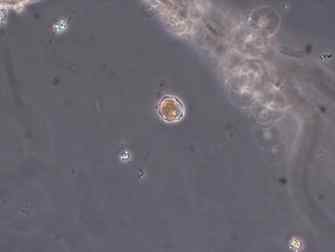
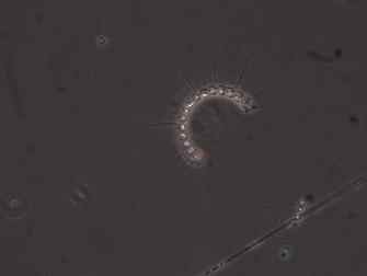
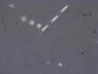
Phytoplankton species (L to R) Alexandrium cantenella, Chaetoceros, Pseudo-nitzchia and Thalassiosira.
Click to enlarge.
Stations 54 and 56 are exposed to direct contact with fresh water influxes streaming into those locations. stations 56 and 54 are fed fresh water from Judd Creek and Fisher Creek respectively. The amount of direct fresh water may influence the type of diversity found in these two stations. As shown in Diagram 1, sampling starting at station 50 and going to station 53, show similar species shared that are not common in the remaining stations going further into Quartermaster Harbor. The commonalities of these 4 stations are the cooler temperatures shown in Figure 1, due to water depth and higher salinity levels due to distance from fresh water influxes. Phytoplankton species common to stations 50-53 are Cylindrotheca, Cosinodiscus and with the exception of station 51, Thalissionema. Inner QMH stations, 54 to 56, share similarities in lower salinity levels, shown in Figure 5, as well as warmer waters due to fresh water influxes and shallow depths. These stations also share phytoplankton species Pseudo-nitzchia, Dinophyllis/physis and with the exception of station 54, Noctiluca. The similarity and differences of the phytoplankton species may be due to differences in salinity. Those that can thrive in different ranges of salinity are euryhaline species, while some can only fully thrive in a specific range of salinity, called stenohaline organisms. Another contributing factor to the difference of species could be due to temperature. The higher temperatures allow an increased rate of biological activity because it allows a faster molecular movement within the cells of organisms. The more diverse species can thrive in a wider range of temperatures which is a characteristic of the eurythermal organisms and those species that can only thrive at a specific temperature belong to the stenothermal organisms. Temperature effects density , in which colder temperatures create an increase in water viscosity. Phytoplankton prefer and thrive more abundantly in warmer less viscous waters which is why the phytoplankton community is more abundant at surface and thermocline depths. It could be assumed from the data that Chaetoceros and Thalassiosira are euryhaline and eurythermal while all other species could be considered stenohaline and stenothermal.
Sediments ( Grain Size )
Graph 2: Sediment graph depicting particle size found in station 52. The graph shows on the (X) axis the particle diameter(um) and on the (Y) axis the volume(%) of the particle size.
Analysis of particle size and volume in station 52 are depicted in the graph above. Nearly 50% of particles were classified in class of 125um.
Graph 3: Sediment graph depicting particle size found in station 53. The graph shows on the (X) axis the particle diameter(um) and on the (Y) axis the volume(%) of the particle size.
Analysis of particle size and volume in station 53 are depicted in the graph above. The mass majority of particle grain size were classified within the range of 63-500um. .
Graph 4: Sediment graph depicting particle size found in station 54. The graph shows on the (X) axis the particle diameter(um) and on the (Y) axis the volume(%) of the particle size .
Analysis of particle size and volume in station 54 is widely distributed among particle size classes 0.4-1000um..
Graph 5: Sediment graph depicting particle size found in one of two samples in station 55. The graph shows on the (X) axis the particle diameter(um) and on the (Y) axis the volume(%) of the particle size.
.Analysis of particle size and volume in station 55 are depicted in the graph above. Nearly 50% of particles were classified in class of 125um.
Graph 6: Sediment graph depicting particle size from second sediment sample found in station 55. The graph shows on the (X) axis the particle diameter(um) and on the (Y) axis the volume(%) of the particle size.
In contrast with first sample of station 55, analysis of particle size is widely distributed among particle classes 0.4-500um..
Total Organic Carbon
Graph 7: Total Organic Carbon found in stations 51-56.
The graph above shows the percent of organic carbon found in each station, with the exception of stations 51 and 52, the total organic carbon increases towards inner harbor. Overall, stations 55 and 56 had a much higher percentage of total organic carbon compared to the other stations.
Station 50 was too deep to obtain a sediment grab, in addition, we were also unable to obtain a sample from station 54.